ATA.Forecast is a generic function for forecasting of the ATA Method.
Usage
ATA.Forecast(
  object,
  h = NULL,
  out.sample = NULL,
  ci.level = 95,
  negative.forecast = TRUE,
  onestep = FALSE,
  print.out = TRUE
)
Arguments
- object
An
ataobject is required for forecast.- h
Number of periods for forecasting.
- out.sample
A numeric vector or time series of class
tsormstsfor out-sample.- ci.level
Confidence Interval levels for forecasting. Default value is 95.
- negative.forecast
Negative values are allowed for forecasting. Default value is TRUE. If FALSE, all negative values for forecasting are set to 0.
- onestep
Default is FALSE. if TRUE, the dynamic forecast strategy uses a one-step model multiple times (
hforecast horizon) where the prediction for the prior time step is used as an input for making a prediction on the following time step.- print.out
Default is TRUE. If FALSE, forecast summary of ATA Method is not shown.
References
#'Yapar G, Yavuz I, Selamlar HT (2017). “Why and How Does Exponential Smoothing Fail? An In Depth Comparison of ATA-Simple and Simple Exponential Smoothing.” Turkish Journal of Forecasting, 1(1), 30–39.
#'Yapar G, Capar S, Selamlar HT, Yavuz I (2018). “Modified Holt's Linear Trend Method.” Hacettepe University Journal of Mathematics and Statistics, 47(5), 1394–1403.
#'Yapar G (2018). “Modified simple exponential smoothing.” Hacettepe University Journal of Mathematics and Statistics, 47(3), 741–754.
#'Yapar G, Selamlar HT, Capar S, Yavuz I (2019). “ATA method.” Hacettepe Journal of Mathematics and Statistics, 48(6), 1838-1844.
Examples
trainATA <- head(touristTR, 84)
ata_fit <- ATA(trainATA, parPHI = 1, seasonal.test = TRUE, seasonal.model = "decomp")
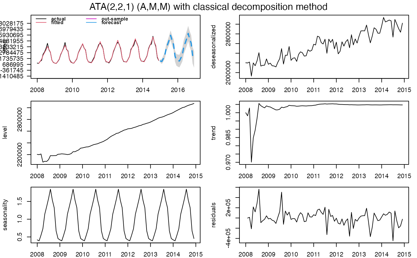 #> ATA(2,2,1) (A,M,M)
#>
#> model.type: M
#>
#> seasonal.model: decomp
#>
#> seasonal.type: M
#>
#> forecast horizon: 24
#>
#> accuracy.type: sMAPE
#>
#> Model Fitting Measures:
#>
#> sigma2 loglik MAE
#> 25327678645.19519043 -1188.55670094 106527.45549230
#> MSE RMSE MPE
#> 23496762116.62686157 153286.53599265 0.12753452
#> MAPE sMAPE MASE
#> 4.04068178 4.04508846 0.23313082
#> OWA
#> 0.00000468
#>
#> In-Sample Accuracy Measures:
#>
#> MdAE MdSE RMdSE MdPE
#> 67333.7563803 4533834748.2853584 67333.7563803 0.4018348
#> MdAPE sMdAPE
#> 3.2125716 3.2275752
#>
#> Out-Sample Accuracy Measures:
#>
#> MAE MSE RMSE MPE MAPE sMAPE MASE OWA
#> NA NA NA NA NA NA NA NA
#>
#> Out-Sample Accuracy Measures:
#>
#> MdAE MdSE RMdSE MdPE MdAPE sMdAPE
#> NA NA NA NA NA NA
#>
#> Information Criteria:
#>
#> AIC AICc BIC
#> 2391.113 2392.587 2408.129
#>
#>
#> user system elapsed
#> 0.081 0.083 0.313
#>
#> calculation.time: 0.3127
#>
#>
#> Forecasts:
#> Time Series:
#> Start = 2015.00694444444
#> End = 2016.92361111111
#> Frequency = 12
#> [1] 1288568 1211322 1716223 2292963 3589547 4283724 5018661 5887346 4933780
#> [10] 4253560 2170497 1480814 1363260 1281536 1815704 2425875 3797616 4532031
#> [19] 5309568 6228607 5219767 4500118 2296310 1566650
#>
#>
ata_fc <- ATA.Forecast(ata_fit, h=12)
#> Time Series:
#> Start = 2015.00694444444
#> End = 2015.92361111111
#> Frequency = 12
#> lower forecast upper
#> 2015 969867 1271754 1573641
#> 2015 768220 1195153 1622086
#> 2015 1169918 1692802 2215686
#> 2015 1657210 2260985 2864759
#> 2015 2863372 3538412 4213452
#> 2015 3481949 4221419 4960888
#> 2016 4145447 4944165 5742884
#> 2016 4944330 5798196 6652062
#> 2016 3951934 4857595 5763257
#> 2016 3231957 4186608 5141259
#> 2016 1134438 2135685 3136931
#> 2016 410853 1456621 2502389
#> ATA(2,2,1) (A,M,M)
#>
#> model.type: M
#>
#> seasonal.model: decomp
#>
#> seasonal.type: M
#>
#> forecast horizon: 24
#>
#> accuracy.type: sMAPE
#>
#> Model Fitting Measures:
#>
#> sigma2 loglik MAE
#> 25327678645.19519043 -1188.55670094 106527.45549230
#> MSE RMSE MPE
#> 23496762116.62686157 153286.53599265 0.12753452
#> MAPE sMAPE MASE
#> 4.04068178 4.04508846 0.23313082
#> OWA
#> 0.00000468
#>
#> In-Sample Accuracy Measures:
#>
#> MdAE MdSE RMdSE MdPE
#> 67333.7563803 4533834748.2853584 67333.7563803 0.4018348
#> MdAPE sMdAPE
#> 3.2125716 3.2275752
#>
#> Out-Sample Accuracy Measures:
#>
#> MAE MSE RMSE MPE MAPE sMAPE MASE OWA
#> NA NA NA NA NA NA NA NA
#>
#> Out-Sample Accuracy Measures:
#>
#> MdAE MdSE RMdSE MdPE MdAPE sMdAPE
#> NA NA NA NA NA NA
#>
#> Information Criteria:
#>
#> AIC AICc BIC
#> 2391.113 2392.587 2408.129
#>
#>
#> user system elapsed
#> 0.081 0.083 0.313
#>
#> calculation.time: 0.3127
#>
#>
#> Forecasts:
#> Time Series:
#> Start = 2015.00694444444
#> End = 2016.92361111111
#> Frequency = 12
#> [1] 1288568 1211322 1716223 2292963 3589547 4283724 5018661 5887346 4933780
#> [10] 4253560 2170497 1480814 1363260 1281536 1815704 2425875 3797616 4532031
#> [19] 5309568 6228607 5219767 4500118 2296310 1566650
#>
#>
ata_fc <- ATA.Forecast(ata_fit, h=12)
#> Time Series:
#> Start = 2015.00694444444
#> End = 2015.92361111111
#> Frequency = 12
#> lower forecast upper
#> 2015 969867 1271754 1573641
#> 2015 768220 1195153 1622086
#> 2015 1169918 1692802 2215686
#> 2015 1657210 2260985 2864759
#> 2015 2863372 3538412 4213452
#> 2015 3481949 4221419 4960888
#> 2016 4145447 4944165 5742884
#> 2016 4944330 5798196 6652062
#> 2016 3951934 4857595 5763257
#> 2016 3231957 4186608 5141259
#> 2016 1134438 2135685 3136931
#> 2016 410853 1456621 2502389