Accuracy Measures for The ATAforecasting

Returns ATA(p,q,phi)(E,T,S) applied to `ata` object. Accuracy measures for a forecast model Returns range of summary measures of the forecast accuracy. If out.sample is provided, the function measures test set forecast accuracy. If out.sample is not provided, the function only produces training set accuracy measures. The measures calculated are:

lik : maximum likelihood functions
sigma : residual variance.
MAE : mean absolute error.
MSE : mean square error.
RMSE : root mean squared error.
MPE : mean percentage error.
MAPE : mean absolute percentage error.
sMAPE : symmetric mean absolute percentage error.
MASE : mean absolute scaled error.
OWA : overall weighted average of MASE and sMAPE.
MdAE : median absolute error.
MdSE : median square error.
RMdSE : root median squared error.
MdPE : median percentage error.
MdAPE : median absolute percentage error.
sMdAPE : symmetric median absolute percentage error.

Usage

ATA.Accuracy(object, out.sample = NULL, print.out = TRUE)

Arguments

object: An object of class ata is required.
out.sample: A numeric vector or time series of class ts or msts for out-sample.
print.out: Default is TRUE. If FALSE, summary of ATA Method's accuracy measures is not shown.

Value

Matrix giving forecast accuracy measures.

References

#'Hyndman RJ, Koehler AB (2006). “Another look at measures of forecast accuracy.” International Journal of Forecasting, 22(4), 679–688.

#'Hyndman RJ, Athanasopoulos G (2019). Forecasting: principles and practice. OTexts. https://otexts.com/fpp3/.

Author

Ali Sabri Taylan and Hanife Taylan Selamlar

Examples

trainATA <-  head(touristTR, 84)
testATA <- window(touristTR, start = 2015, end = 2016.917)
ata_fit <- ATA(trainATA, h=24, seasonal.test = TRUE, seasonal.model = "decomp")

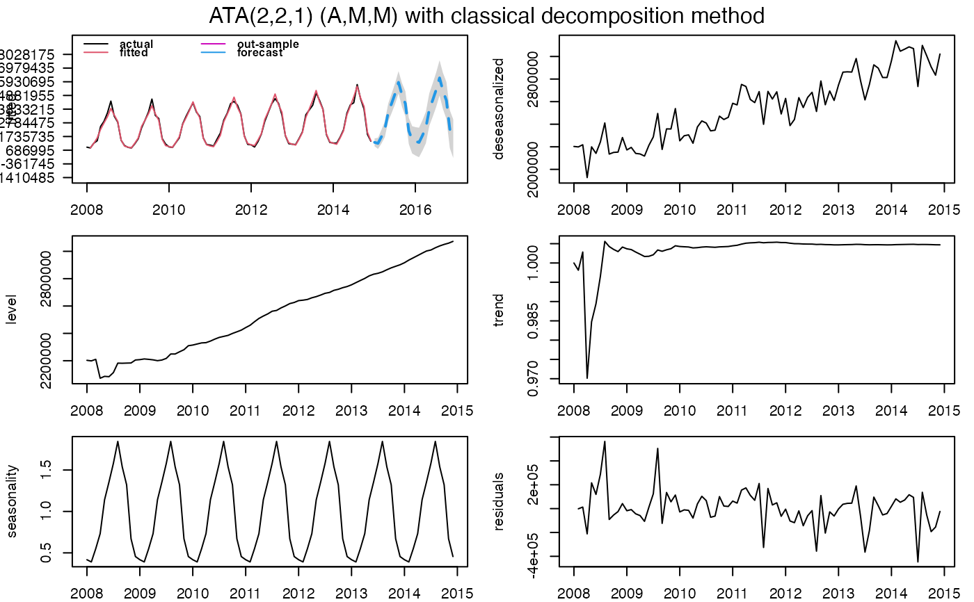#> ATA(2,2,1) (A,M,M) 
#> 
#>    model.type: M 
#> 
#>    seasonal.model: decomp 
#> 
#>    seasonal.type: M 
#> 
#>    forecast horizon: 24 
#> 
#>    accuracy.type: sMAPE 
#> 
#> Model Fitting Measures: 
#> 
#>               sigma2               loglik                  MAE 
#> 25327678645.19519043       -1188.55670094      106527.45549230 
#>                  MSE                 RMSE                  MPE 
#> 23496762116.62686157      153286.53599265           0.12753452 
#>                 MAPE                sMAPE                 MASE 
#>           4.04068178           4.04508846           0.23313082 
#>                  OWA 
#>           0.00000468 
#> 
#> In-Sample Accuracy Measures: 
#> 
#>               MdAE               MdSE              RMdSE               MdPE 
#>      67333.7563803 4533834748.2853584      67333.7563803          0.4018348 
#>              MdAPE             sMdAPE 
#>          3.2125716          3.2275752 
#> 
#> Out-Sample Accuracy Measures: 
#> 
#>   MAE   MSE  RMSE   MPE  MAPE sMAPE  MASE   OWA 
#>    NA    NA    NA    NA    NA    NA    NA    NA 
#> 
#> Out-Sample Accuracy Measures: 
#> 
#>   MdAE   MdSE  RMdSE   MdPE  MdAPE sMdAPE 
#>     NA     NA     NA     NA     NA     NA 
#> 
#> Information Criteria: 
#> 
#>      AIC     AICc      BIC 
#> 2391.113 2392.587 2408.129 
#> 
#> 
#>    user  system elapsed 
#>   1.799   0.545   3.834 
#> 
#> calculation.time: 3.8347 
#> 
#> 
#> Forecasts: 
#> Time Series:
#> Start = 2015.00694444444 
#> End = 2016.92361111111 
#> Frequency = 12 
#>  [1] 1288568 1211322 1716223 2292963 3589547 4283724 5018661 5887346 4933780
#> [10] 4253560 2170497 1480814 1363260 1281536 1815704 2425875 3797616 4532031
#> [19] 5309568 6228607 5219767 4500118 2296310 1566650
#> 
#> 
ata_accuracy <- ATA.Accuracy(ata_fit, testATA)
#> Model Fitting Measures: 
#> 
#>               sigma2               loglik                  MAE 
#> 25327678645.19519043       -1188.55670094      106527.45549230 
#>                  MSE                 RMSE                  MPE 
#> 23496762116.62686157      153286.53599265           0.12753452 
#>                 MAPE                sMAPE                 MASE 
#>           4.04068178           4.04508846           0.23313082 
#>                  OWA 
#>           0.00000468 
#> 
#> Out-Sample Accuracy Measures: 
#> 
#>                    MAE                    MSE                   RMSE 
#>        745266.93257918 1268723834847.21044922       1126376.41792041 
#>                    MPE                   MAPE                  sMAPE 
#>           -28.69225078            29.56321404            23.01067141 
#>                   MASE                    OWA 
#>             1.63098511             0.00002695 
#> 
#>